Ledidi

Statistics are indispensable when trying to understand the world around us. They help us use data to answer questions, recognise patterns, associations, and causations, generate new insights and knowledge - and often point us towards further questions to ask. In healthcare, statistics are vital to generating the knowledge we need to improve the quality of care and develop new therapeutic solutions.

Within statistics, there are two main approaches to data analysis: descriptive and inferential statistics. Where descriptive statistics allow you to explore, describe and summarise your data, hypotheses can be tested and conclusions drawn using inferential statistics. In this article, we will take a closer look at these two approaches and see how and when they are appropriate to use.

Descriptive statistics

The first step in your data analysis should always be to perform some descriptive statistics. This process is often called “exploratory data analysis”. Here one explores a dataset in a relatively unstructured way. The goal is not to test a hypothesis, as is the case with inferential statistics, but to obtain greater insight into your data, and uncover patterns, and even potential issues. In short, descriptive statistics enable us to present our data in a meaningful way allowing simpler interpretation.

There are different types of descriptive statistics including measures of central tendency, frequency, dispersion/variation, and position.

• Measure of central tendency includes mean, median, and mode. This indicates the distribution of the variable(s) and is used for numerical variables.

• Measure of frequency includes frequency, ratio, rate, proportion, and percentage. These measures describe how often a value occurs and is used for categorical variables.

• Measure of dispersion/variation includes range, variance, and standard deviation. This identifies the spread of the values and is used for numerical variables.

• Measure of position includes percentile ranks and quartile ranks. This describes where values fall in relation to each other and is used for numerical variables.

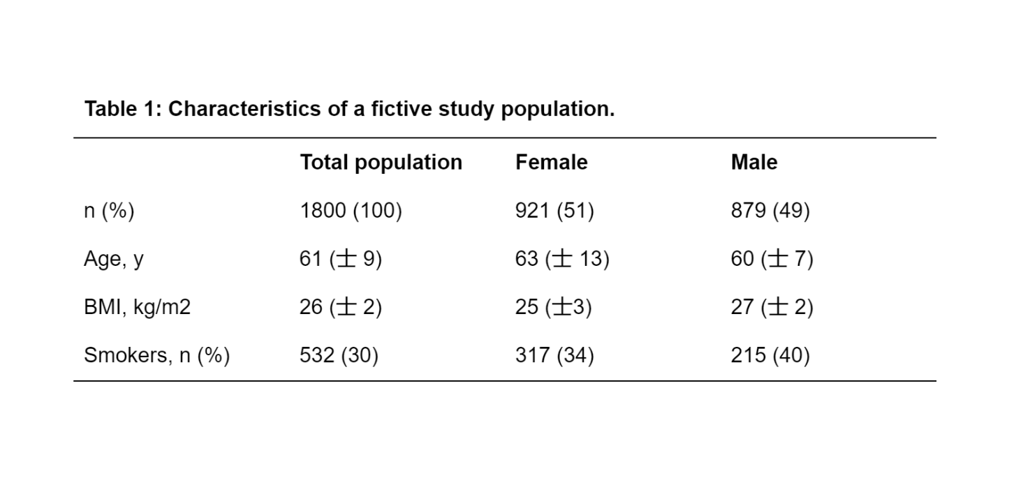
Typically, in a scientific publication, the results of a descriptive statistical analysis are depicted in the first result table (often called “Baseline table”). This is not only essential for the researcher to obtain insight into the dataset, but also for any potential reader to quickly get an overview of the data material used in the study. An example is shown below in Table 1.

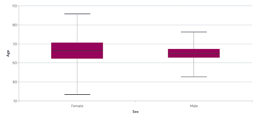
Reporting descriptive statistics can be done using tables, as shown above. However, a graphical representation is often equally appropriate. The optimal way of graphically presenting your data depends on the variable type and whether the analysis is univariate (one variable at a time) or multivariate (two or more variables at a time). Figure 1 depicts the same data as in table 1 in a boxplot (mean age in the female and male groups).

A summary of which descriptive statistics to use and a possible graphical presentation per variable and analysis type is given in the matrix below.

One limitation of descriptive statistics is that its results are only applicable to your study sample and cannot be extrapolated to the whole population. To generalize results from a sample to a population, the use of inferential statistics is necessary.

Inferential statistics

In situations where the aim of the study goes beyond just describing a certain sample, we move on to inferential statistics after the initial exploratory analysis. Inferential statistics is a collective term for methods used to draw conclusions on a population from which we obtained a sample (as we often only investigate part of a population, i.e. a “sample”, and not the entire population at once). They are based on the fact that sampling error is innate to the sampling process leading to a sample not perfectly representing the population.

The methods used can be divided into two major areas:

• Testing of statistical hypotheses

• Estimation of parameters

Testing of statistical hypotheses

When conducting research, you are inevitably trying to answer a research question or a hypothesis that you have set. As an example, let’s say you want to investigate the association between trans fat intake and heart infarction. There are many ways of formulating a hypothesis but it should at least contain:

• the relevant variables (e.g. Trans fat and heart infarction)

• the predicted outcome of the experiment or analysis or the proposed relationship between the variables (e.g. positive association between trans fat intake and risk of developing heart infarction)

• the specific group being studied (e.g. patients with established cardiovascular disease)

Your hypothesis should be testable and specific: “The intake of trans fatty acids is positively associated with an increased risk of experiencing a heart infarction in patients with established cardiovascular disease”.

It is also necessary to formulate a null hypothesis i.e. the default assumption that there is no relationship between the variables of interest. In our example, the null hypothesis would be: “The intake of trans fatty acids is not associated with risk of experiencing a heart infarction in patients with established cardiovascular disease.”

After hypothesis formulation and data collection, it is time to test the hypothesis using statistical testing. To choose the appropriate test, it is essential to know your data: the different variable types and if they meet certain assumptions which vary according to the statistical test used. These tests can provide a wide variety of insights into your data (e.g. the probability that you would get the obtained results if your hypothesis was actually wrong (p-value) or how much one variable changes depending on changes in a different variable (beta coefficient)) depending on the used test. Interpreting these results is not always straightforward and should be done carefully.

For more information regarding hypothesis testing and interpreting the results, read our “P-values”, “Parametric vs non-parametric tests” and “The difference between association, correlation, and causation” articles.

Estimation of parameters

The properties of a population, such as the population mean or median, are called parameters since they represent the whole population. Properties of samples, however, are not called parameters but statistics. Inferential statistics allow us to take statistics from sample data (e.g. x% higher risk of having a heart attack per increase in x grams of consumed trans fat) and use them to make generalizations, or “inferences” about a population parameter (e.g. all cardiovascular patients have an x% higher risk of having a heart attack when eating a certain amount of trans fat).

This assumes the sample is an accurate representation of the population and highlights the importance of a proper sampling strategy. However, inferential statistics are based on the fact that sampling inevitably generates sampling error leading to the sample not being a perfect representation of the population.

This causes one of the main limitations regarding the use of inferential statistics. The provided data is about a population that is not fully measured and one can therefore never be completely sure that the calculated values/statistics are correct. This leads to the second limitation, namely that some statistical tests require the making of assumptions to run them. This again entails uncertainty, which will have consequences for the certainty of the results of the statistical tests.

Data analysis is essential for any type of scientific research. Knowing which statistical analysis to use in which situations is not only good research practice but also allows for reporting appropriate results in a systematic manner. Descriptive statistics should always be the first step as it provides valuable insight into your data. Do you want to make predictions from your data? Inferential statistics is the tool you need.