Ledidi

Mean, median and mode are all commonly used in descriptive statistics (read more about descriptive statistics here). These measures have in common that they are used to indicate the distribution of the variable(s) and try to summarize your dataset with a single number to represent a “typical” data point from your dataset. The different measures are calculated in different ways and have different use areas. In this article, we will go through both how these measures are calculated and the appropriate use, but in short:

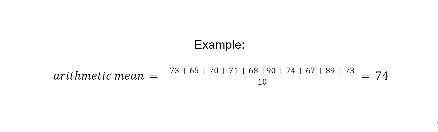
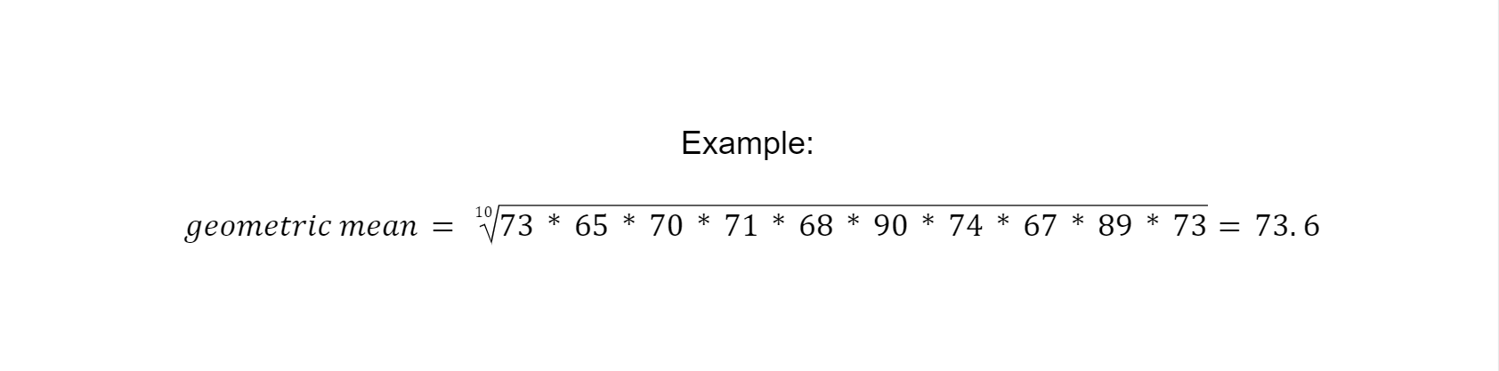
To illustrate the different measures, we will use a small fictional dataset including the weight of 10 individuals as an example:

• Mean is the average value of the data points (observations
• Median is the value that is exactly in the middle when all values are arranged from low to high
• Mode is the value which occurs most frequently in your dataset

To illustrate the different measures, we will use a small fictional dataset including the weight of 10 individuals as an example:

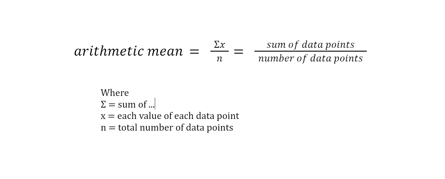
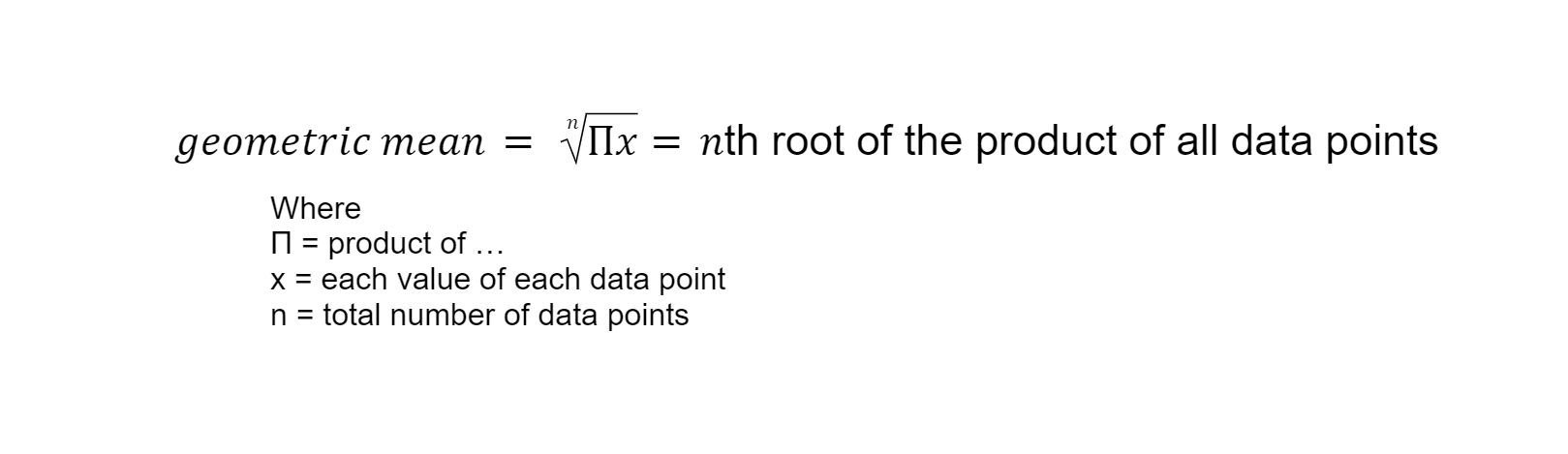
Mean

The mean can be calculated both as the arithmetic mean and as the geometric mean.

The arithmetic mean, often referred to simply as “mean”, is the average value of all data points. It is calculated by adding the values of all data points and dividing them by the number of data points.

The geometric mean is also the average value of data points, just like the arithmetic mean. However, to calculate the geometric mean, one must calculate the nth root (with n = total number of data points) of the product of all data points.

Median

The median of your data points is the value that is exactly in the middle when all values are arranged from low to high. When your dataset has an even number of observations, so there is no value exactly in the middle, calculate the mean of the middle two values.

Example:

1. Arrange all values from high to low
   65 67 68 70 71 73 73 74 89 90

2. Find the middle value. NB: Our dataset has an even number of observations, so we will calculate the mean of the middle two values.
   65 67 68 70 71 73 73 74 89 90

→ Median = 72

Mode

The value which occurs most in your dataset is called the mode. Depending on your dataset, there can be no, one, or several modes. The mode can be found by selecting the value that occurs the most. While the mode can be used for numeric data, it is the one measure of central tendency which can also be used for categorical data.

Example:

First, let’s find the mode for our numerical dataset. The only number which occurs more than once is 73. So the mode in our example dataset is 73.

Now, when we categorize our individuals according to their BMI as “underweight”, “normal weight” and “overweight”, we get a new dataset with categorical data.

To find the mode, creating a frequency table might be helpful.

→ Mode = Normal weight

Visualisation

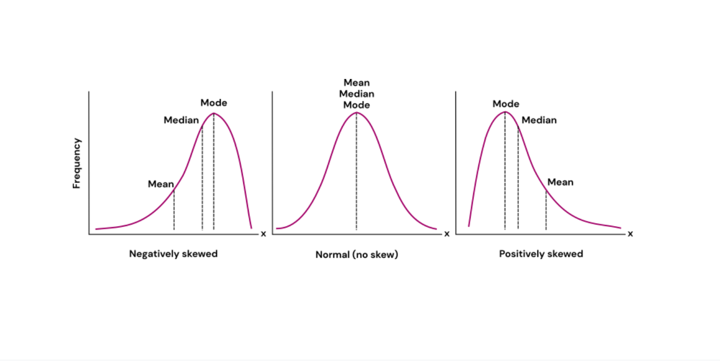
For normally distributed data, the mean, median, and mode will have the same value. This is not the case for skewed data. Figure 1 shows where the mean, median, and mode of your dataset are located for different distributions.

When to use mean, median, or mode?

Which measure of central tendency to use depends mainly on two things:

1. The variable type
2. The shape of your distribution

For categorical variables, there are no numerical values, so the mean cannot be calculated. In this case, the mode is the best measure of central tendency as it tells you which value appears most commonly in your dataset.

However, for numerical variables (continuous or discrete variables), both the mean and the median can be calculated. So, when to use which? Here, the shape of your distribution becomes important.

As mentioned earlier, when your data is normally distributed, the mean and median will have the same value. However, for skewed distributions, i.e., when one side of the distribution is more spread out and has a longer tail than the other, it is best to use the median. This is because the mean is influenced by extreme values (or “outliers”) and might therefore not be a good representation of a “typical” value of your dataset. Because the median takes a value from the middle of the distribution, it is not as influenced by extreme values and will therefore be a better measure of central tendency.

Arithmetic or geometric mean?

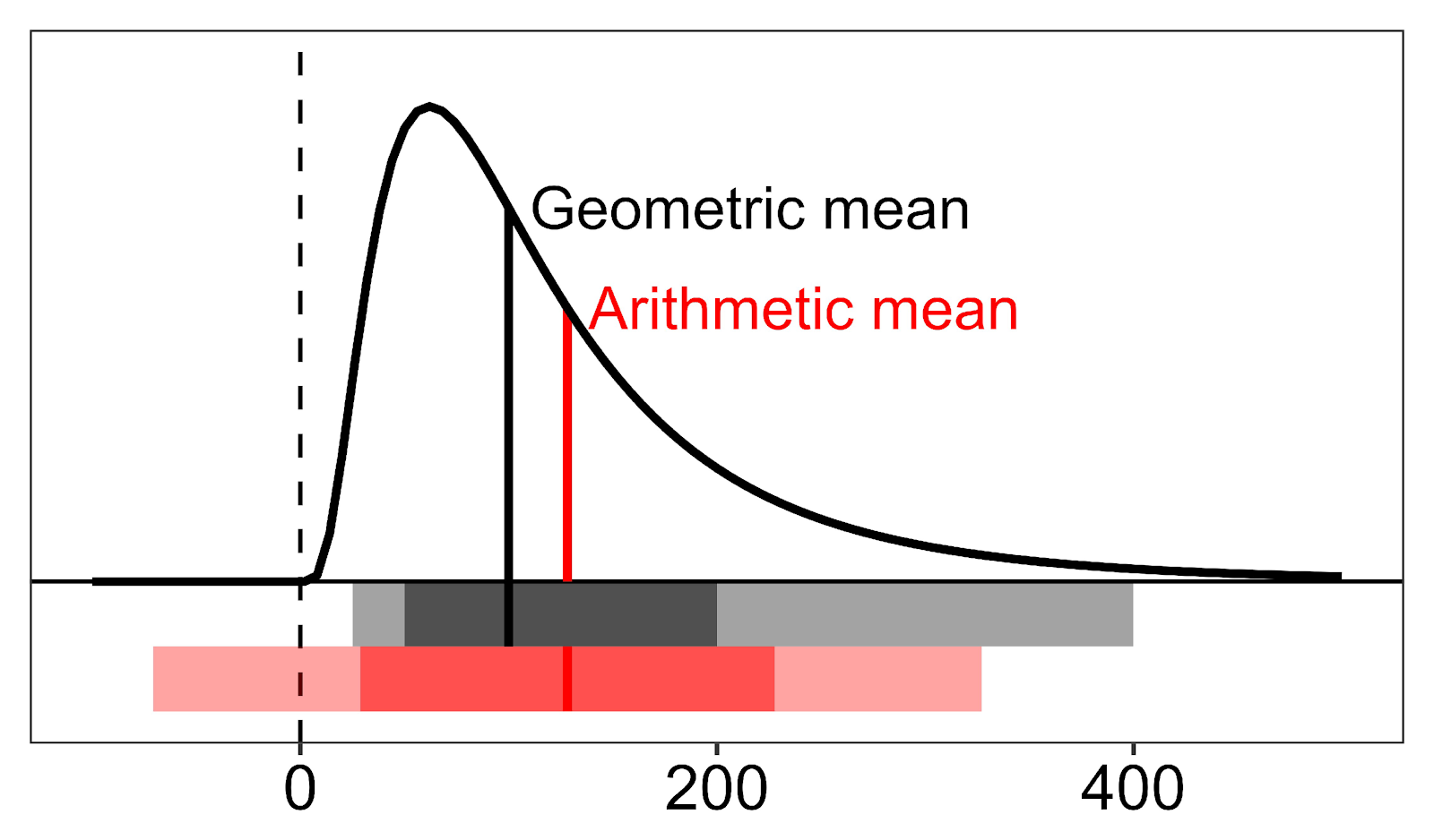
The geometric mean is suggested to be a better representative of log-normal distributions and percentages. Log-normal distributions are skewed, but after logarithmic transformation, they become normally distributed. These distributions typically have a high number of similar values with few extreme values and are common for biological measurements. For this type of distribution, the arithmetic mean is pulled upward due to the outliers, therefore, the geometric mean tends to be lower and represents smaller values better (See Figure 2).

Commonly, biological values have a true zero (meaning their value is actually zero) and do not take on a negative value (e.g., it is not possible to have negative blood pressure or plasma insulin). This is an important fact when it comes to calculating the standard deviation (SD).

Typically, an interval within ± 1 SD from the mean covers about 68% of the distribution, while an interval within ± 2 SD covers about 95%. As shown in Figure 2 in red, for the arithmetic mean this interval spans too low below the mean and can contain zero and negative values, which is biologically impossible. Additionally, the interval doesn’t span high enough above the mean. However, this is not true for the interval covered by one or two geometric SD from the geometric mean.

If you have a skewed distribution for your measurements, it is most likely more correct to report the geometric mean and its corresponding SD instead of the arithmetic mean.

How to calculate these measurements in Ledidi Core

(Arithmetic) mean & median
When calculating the (arithmetic) mean and median of just one variable, the “Explore” analysis is what you need.
Not sure how to run this analysis?
Watch our How-to video!

If you want to calculate the mean and median of one variable across several groups at once, use the “Compare numeric values” analysis.
This How-to video shows you how that’s done.

Mode
The mode for categorical variables can easily be found by creating a frequency table using the “Frequencies” analysis.
This How-to video explains how that can be performed in Ledidi Core.