
The increasing controversy surrounding the use and reporting of p-values (1), (2) does not take away from the p-values’ status as one of the most reported statistical measures. However, although widely used in several fields utilizing quantitative research methods, a surprising number of researchers and other professionals will have trouble explaining what information the p-value really gives.
First, we can address a common misinterpretation from the get-go: The p-value does not equal neither degree of truth nor correctness of a finding. It would be easy to assume that a p-value >0,05 means that your hypothesis is wrong/there is no difference between study groups, while a p-value <0,05 means that your hypothesis is correct/there is a difference between study groups; yet this is overly simplified and not entirely correct.
So, how can we define the p-value in a correct, useful, and memorable manner?
The (very) short version
The p-value is the probability that you would get the result obtained, or an even more extreme result, if your hypothesis was actually wrong.
The more elaborate version
To really understand the correct definition and interpretation of a p-value, one needs to have some understanding of the concept of hypothesis testing.
Quantitative research mainly consists of hypotheses that are being tested. The research question, if not already stated as such, can be rather easily converted to a hypothesis by changing the question to a statement. This statement will be true or untrue, which is what we try to find out through measurements and statistics.
Let us say that the research question is “Is there a difference between two groups?”. Converting this to a statement, we get the hypothesis: “There is a difference between the two groups”. To test it statistically, we must compare it to the opposite possibility; that there is no difference between the groups. In research methodology, this opposite, “no difference”, hypothesis has been given the name null hypothesis (H0). An easy way to think of this is that it represents a null result/null finding.
So, if the research question is “Is there a difference between the reading skills of 7-year-olds in New York vs Boston?”, then the hypotheses being tested would be:
Hypothesis: There is a difference in reading skills.
Null hypothesis: There is no difference in reading skills. (Or, stated otherwise, reading skills are the same.)
We then test the reading skills of a sample of 7-year-olds from both cities and compare them mathematically. If we find that the 7-year-olds in Boston on average score 0.45 points higher that the New York kids, on a scale from 1-5 (ie, 4.10 vs 3.65); would it then be correct to conclude that 7-year-olds in Boston are 12,3% better at reading?
As we have only tested a sample of the eligible children, we could have randomly - and completely by chance - picked out a larger proportion of excellent readers in Boston than in New York, even if the over-all reading skills were identical. The p-value obtained from running a more sophisticated analysis than just comparing means, will indicate whether we can trust the result:
The obtained p-value is the probability that we would, by chance, measure an average difference of 0.45 points or more if the reading skills are actually identical between 7-year-olds in the two cities.
Hence, a low p-value indicates that it is unlikely that we would get a difference as high as 0.45 if there is no difference at all. Conversely, a high p-value indicates a high probability that the measured difference has happened by chance, and not due to an actual difference.
Statistical tests
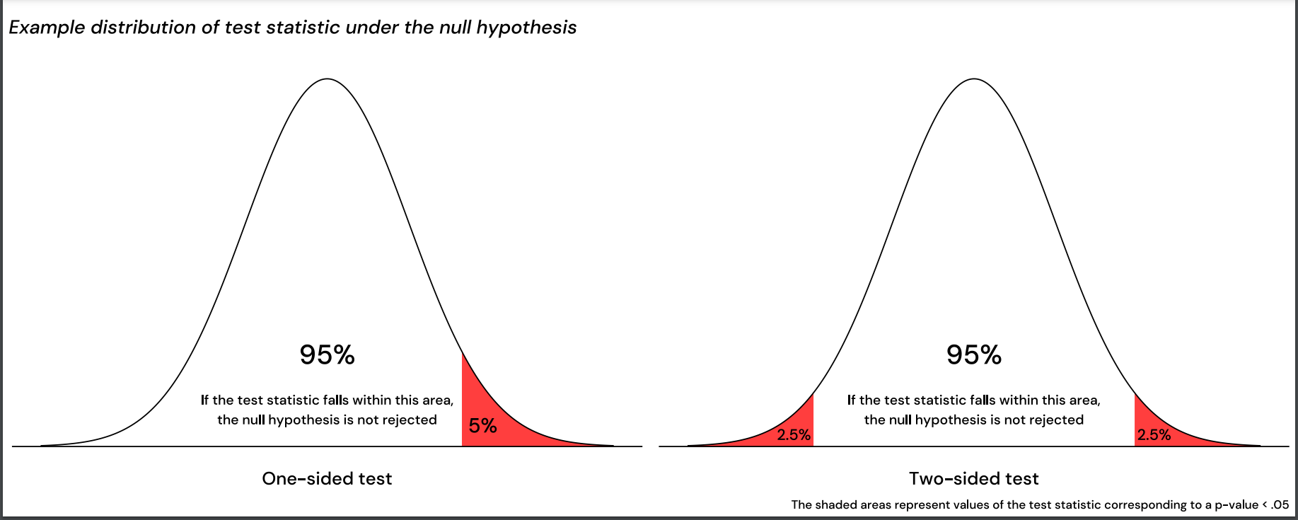
There are a wide range of statistical tests available, which all yield p-values to indicate statistically significant relationships between variables or differences between groups. Common for these tests, is that they mathematically compare the observed values with the range of values predicted from the null hypothesis (the values one would expect from a null finding) by use of a so-called test statistic. The test statistic has an expected distribution under the null hypothesis, which for example resembles a normal curve for some common statistical tests; see Figure 1. If the test statistic has a more extreme value than 95% of this “null distribution”, the p-value will be less than 0.05, and one would reject the null hypothesis.
To choose the right statistical test, so that the observed values are compared to the correct distribution of predicted “null values”, you need to know your data: What types of variables you have (quantitative or categorical, ordered/non-ordered, etc.), and if they meet certain assumptions, as some statistical tests have stricter requirements than others. Some common assumptions are that the data are normally distributed, that the variance is similar between compared groups, and that there is independence between the observations. If the data do not follow the normal distribution or the variance is heterogenic, one can use so-called non-parametric tests, as these tests contain no assumptions about the data distribution. The trade-off is that these tests might have less statistical power; meaning, the probability to be able to reject an untrue null hypothesis is lower. There are several flow charts available to help guide the decision on which statistical test is best suited for your data and research question.
Read more about which test to choose in different settings in this article: Parametric versus nonparametric tests
One-sided or two-sided tests
Another decision that needs to be made when comparing two groups, is whether to use a one-sided (one-tailed) or two-sided (two-tailed) statistical test. The difference, in short, is whether you are interested in knowing about any difference in either direction, or if it is only one direction that is interesting. With reference to the distribution of the test statistic illustrated in Figure 1: With a two-sided test, the null hypothesis will be rejected if the test statistic falls in either tail of the curve, while only a value in either the upper OR lower tail would reject the null hypothesis with a one-sided test.
In the example above, a two-sided test would detect any potential difference between students in the two cities, while a one-sided test would only detect if one predetermined group was better than the other. If the data showed the opposite, the null hypothesis would not be rejected, regardless of however big the difference could be in the opposite direction.
The hypotheses as stated above would apply to a two-sided test:
Hypothesis: There is a difference in reading skills.
Null hypothesis: There is no difference in reading skills. (Or, stated otherwise, reading skills are the same.)
With a one-sided test, the hypotheses must be formulated differently:
Hypothesis: 7-year-olds in New York have better reading skills than 7-year-olds in Boston.
Null hypothesis: 7-year-olds in New York does not have better reading skills that 7-year-olds in Boston (including both the possibility of no difference, and that the children in Boson might have better reading skills.)
A one-sided test has the advantage of more statistical power; hence, one is more likely to detect a difference if it is in the expected direction. But there are some requirements that should be met: One must decide on the direction before looking at the collected data, and the direction should be obvious. For instance, if one is testing a more powerful battery in an electric car, one can be fairly certain that the car’s distance range will not decrease. But one particular direction being the desirableoutcome is not a valid reason to choose a one-sided test. Second, it must be decided that a finding in the opposite direction of the expected would be completely uninteresting and discarded as a finding by chance, no matter how big a detected difference might be. For these reasons, one-sided tests should be used with caution, and one must be ready to defend the choice when publishing the results.
Be cautious
For practical purposes, a p-value cut-off of <0.05 for statistical significance is often used in research papers. This means that a result is accepted when the probability of it being caused by chance is less than 5%. However, when performing two tests, the probability that one of them is caused by chance doubles to 10% if the individual cut-off is kept at <0.05. This probability further increases with the number of tests: Statistically, if there is no true effect or difference, the probability that one in twenty tests would yield a p-value <0.05 reaches towards 100%. Because of this, it is appropriate to use methods to adjust for multiple testing, especially when working with big data. One simple and common method is the Bonferroni adjustment, which calculates a dataset specific cut-off value by dividing the preferred significance level (ie. 0.05) by the number of tests performed.
It is also important to keep in mind that p-values are strongly affected by the sample size. Given that the measured, average difference remains the same, the p-value would decrease for each extra observation. Which makes sense: If we knew that 1000 children in each city had been tested in the example above, we would intuitively trust the result more than if only 10 were tested and expect a lower p-value. If there was no true difference between the groups, however, then the measured difference would inevitably decrease with increasing sample size. A difference observed from a large proportion is hence more trustworthy, which is reflected in the p-value.
Importantly, given a sufficiently large sample size, even the smallest of differences would yield significant p-values. One must thus keep in mind that the p-value says nothing about the relevance of a finding.
The p-value also does not indicate the reliability of the measured effect size. For this, the 95% confidence interval is much better suited. As this interval also intrinsically indicates statistical significance, it is increasingly recommended to avoid focusing on p-values, and rather report the 95% confidence intervals instead.
References
1) Amrhein V, Greenland S, McShane B. Scientists rise up against statistical significance. Nature 567, 305-307 (2019)
2) Ronald L. Wasserstein & Nicole A. Lazar (2016) The ASA Statement on p-Values: Context, Process, and Purpose, The American Statistician, 70:2, 129-133, DOI: 10.1080/00031305.2016.1154108
The p-value is one of the most reported statistical measures within quantitative research, hence it’s crucial to know how to interpret it correctly.
More From Ledidi Academy


The difference between association, correlation and causation
- Statistical analysis
- Tips and insights